《奥本海默》
声明
本文不讨论任何政治观点,内容仅限于《奥本海默》电影本身及其所涉及的历史事实,本文涉及部分剧透内容,请还未观看该电影的朋友酌情阅读。愿世界和平。
正文
“我现在成了死神,世界的毁灭者”——《薄伽梵歌》
上世纪五十年代,随着曼哈顿工程的成功,宣告着人类正式迈入原子能的新纪元,人类首次使用原子能就是曼哈顿工程所创造的「原子弹」,《奥本海默》这部电影就是在讲述原子弹的诞生和原子弹之父奥本海默的故事,全片「181 分钟」作为我个人观看的时间最长(实际上「复联 4」会比它长 1 分钟)的一部电影,对我来说产生了深刻的思考。
它不像一部传统的「阿美利卡」个人英雄主义电影(参考漫威系列),它是一部高唱着和平与现实的的电影,这当然有「基于事实所拍摄的电影」这样的因素在内,虽然我们都知道是奥本海默缔造了「原子弹」,也因此被称为原子弹之父,但是我们都知道「原子弹」不是奥本一人的成果,而是那个历史上所有物理学家、数学家、化学家的杰作,是他们引领人类走进了原子能时代,而奥本海默是一位跨学科的人才,只有这样的跨学科的人才才能够将历史上所有的研究串通起来,完成这个跨越了数学、物理、化学、军事的任务。
我想我们应该庆幸创造了「原子弹」的科学家们都足够有良知,正如奥本海默所引用的那段梵语一样,也正如奥本海默会见杜鲁门所说:“我们科学家的双手沾了血”,「原子弹」的成功让这帮物理学历史上最闪耀的群星开始怀疑自己的研究,我们从历史后来者的角度来看待这些问题,这些科学家,特别是以奥本海默为首的科学家,极力阻止氢弹的开发,阻止原子能更大规模的武器化,就连当初给罗斯福写信劝说上马曼哈顿计划的爱因斯坦都或多或少的在阻止恐怖的事情发生。
说到爱因斯坦,不得不感叹,在那个年代,作为世界上最顶级的物理学家,全世界除了波尔难逢对手,电影里有个片段,奥本海默为了解决「原子弹」有可能的风险问题而去寻找爱因斯坦的帮助,不过爱因斯坦并没有伸出自己的援助之手,至于原因,则是一些比较有趣的故事,显然奥本海默是更相信哥本哈根诠释的,不然也不会多次希望见到波尔,当然除此之外,我想另一方面还是爱因斯坦相信奥本海默可以解决这个问题。不过呢,就真的要感叹,即使是奥本海默被誉为原子弹之父,还有世界上那么多杰出的物理学家,都不得不生活在他的笼罩之下,需要寻求他在学术上的帮助,足以证明爱因斯坦在物理学上有多么不可撼动的实力了。
我们不评价这群创造了「原子弹」的科学家他们的努力阻止之后对后世的影响,因为我想从另一个角度来看这个他们,尤其是奥本海默此人。 在电影中,由小罗伯特唐尼扮演的刘易斯・斯特劳斯算是一位电影里的反派角色,但是他的话也足以让人深思,我们要讨论的就是,奥本海默是否在成为原子弹之父拯救了一次世界之后,又扮演了一个反对原子能进一步武器化的人,想又一次成为救世主呢?说的难听一点,颇有一种当了婊子立牌坊的风味在内了,但是我们无法得知他是否是这样想的,但是我们从科学精神上来思考这件事,我想斯特劳斯的想法是极大的错误,他对物理的了解只是很浅薄的,他不具有科学精神,他具有的是某些令人发指的精神,而科学就当是无国界的,我们发展科学的目的也是为了更好的生存、生活,而不是毁灭生活甚至生存的权力,或许这就是奥本海默所想的,但是这只是我的猜测。
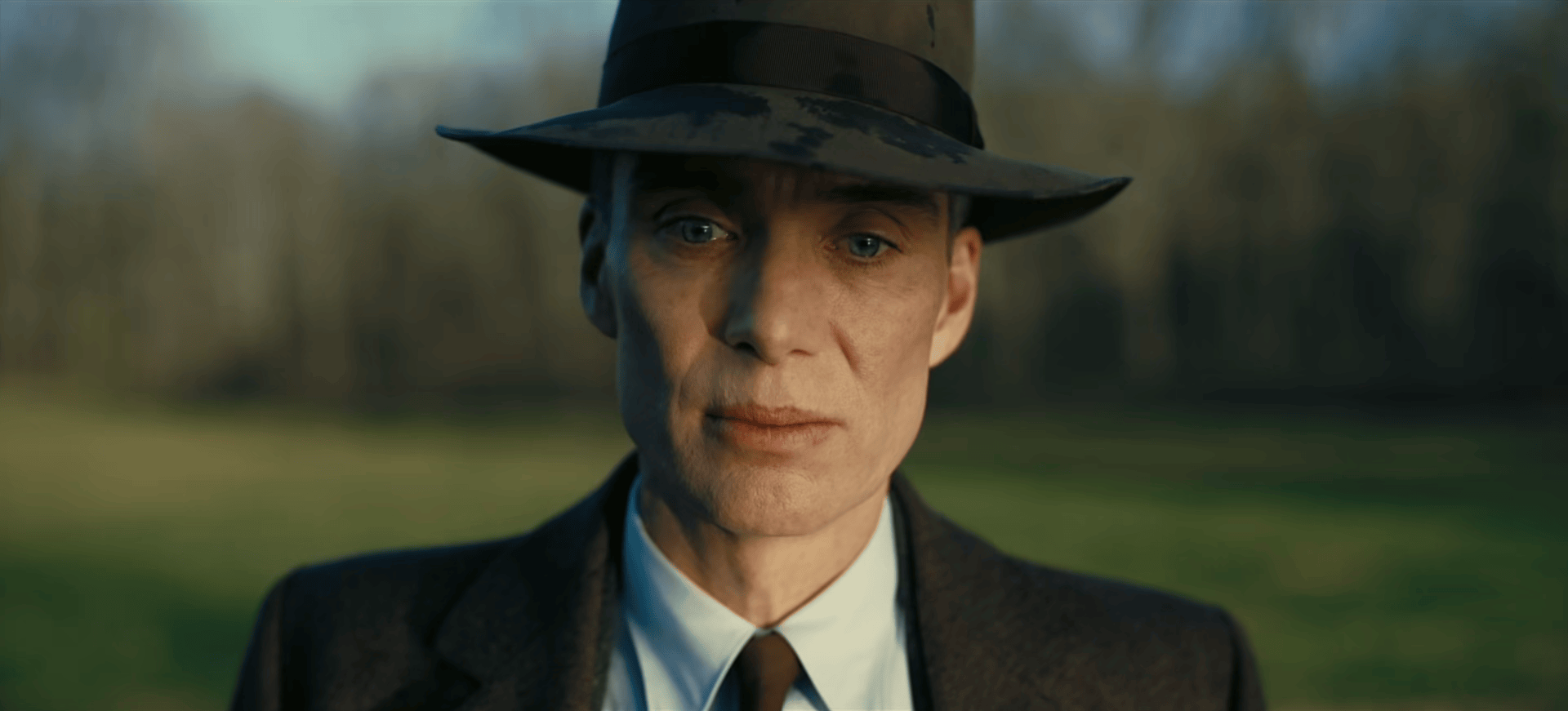
电影在「原子弹」爆炸后,给了奥本海默许多十分有深意的镜头,这些镜头呈现出了复杂的内心,他已经接受了原子弹之父的称呼,但他似乎并不能接受如此巨大的牺牲。
从电影的叙事手法上来讲,它使用了交叉叙事的方式,如此的叙事方式会让本身很简单的历史故事,变得有些「烧脑」,但是也让本来会让人觉得索然无味的电影变得有趣了起来,我想这也是一种不错的文学叙事方式,但是文学上面的话可能会需要淡化一点,否则会对整个作品造成割裂感。
全片在叙事方面,在刘易斯・斯特劳斯的镜头里或者说在叙述对奥本海默不利的内容时,都使用了黑白镜头,而其它大部分都是彩色镜头,这也让电影变得很有意思,在如今的大部分作品里,使用黑白镜头的作用都是在讲述过去的事情,亦或者是特意造景,想要凸显某种特征性的元素,使作品更具有冲击力,当然,假若用意为后者,那么通常都是某些篇幅较小的微电影中,并不会或者说很少出现在如此的商业电影之中,而诺兰导演的如此的设计着实会让人觉得眼前一新,而他使用黑白镜头的用意是什么?这是一个很好的问题,对此有人认为,黑白镜头代表了一种客观的,他人视角的故事,而彩色镜头则是在讲述奥本海默的传奇故事。这样的说法确实很有说服力,而我在北京电影学院编导系的朋友所说的和这样的看法是很类似的,就是以第二个视角来看待奥本海默的所作所为。
在技术方面,我们都知道这部电影使用了 IMAX 胶片相机进行拍摄,这使得这部电影在 IMAX 影厅的呈现会远超大部分所谓的 IMAX 电影,表现十分惊艳,之所以是「所谓」很大部分原因是,这些电影并没有使用 IMAX 相机进行拍摄,就比如我们熟知的《流浪地球 2》、《封神》这两部电影,他们都有在 IMAX 影厅上映,但是画面都有一定的裁切,使得 IMAX 的呈现效果并没有想象的那么好,当然了,虽然画面上比不上《奥本海默》,但是它的音效在 IMAX 影厅有非常好的表现,这当然是因为它的实现难度并不高,而且普通电影机的驾驭难度会远远低于 IMAX 机器。
我们都知道,假若以全画幅为标准,一般情况下我们使用的「残幅」换算成全画幅的等效焦距,需要在焦距上都需要乘以一个大于 1 的数来进行换算,就比如 索尼 的 APS-C 画幅换算为全画幅的等效焦距,要乘的数大概是 1.5 左右,比如一个 50mm 的镜头在 APS-C 的实际表现是 75mm 左右的焦距,这会使得画面得到大比例的裁切,这对新手来说不见的是一件坏事,因为他更方便构图,不过很多人为了在同样的焦距下获得更广的画面而选择了全画幅,(不同的焦段负责不同的任务,这里不再过多讲述)但是对于影视行业来说,更小的画幅能够更好构图,也能够剩下更多的布景经费,但是这样在影院的呈现就会一塌糊涂,而且在部分场景的呈现表现也会很差劲,因此影视人都选择采用全画幅相机进行拍摄,而 IMAX 相机是反其道而行之,它换算为全画幅等效焦段,需要乘以一个小于 1 的数,这使得我们同样使用 50mm 镜头进行拍摄,所获得的内容数量是 IMAX>全画幅>残幅 的,这也是为什么 IMAX 电影可以有更好的画面呈现效果,当然这只有在 IMAX 影院,屏幕使用了 IMAX 特定的屏幕比例才会有的效果,没有使用 IMAX 相机进行拍摄的电影在后期是很难或者说几乎不可能制作出和 IMAX 相机同样的效果。
这部电影无论是从内容上来讲还是技术上来讲都堪称一流,在豆瓣上也获得了 8.6 分的成绩,分数相对诺兰本人的《星际穿越》和《盗梦空间》是低了一些,因为电影本身所讲述的故事只是一个原子弹之父的传奇故事,仅此而已,它并不具备上面这两部电影带给观众们的震撼,而且交叉叙事的方式会很烧脑,把部分观众搞得云里雾里,有人对它的时长并不喜欢,毕竟「181 分钟」的故事会让全片显得有些冗长,当然还有人对奥本海默本身的故事并不喜欢。
总的来说,这部电影十分优秀,足以引人深思,也有足够的视觉震撼,甚至高唱了时代主旋律,一个来自大洋彼岸的电影有如此高的觉悟,真的是难能可贵的。
过于强大的力量可以用于保护,也可以用于摧毁。
特别鸣谢
ZZT —— 北京电影学院广播电视编导系在读
QQ 老冰 —— 摄影爱好者、音频爱好者、我的爱人
参考资料
《奥本海默》电影全片
流浪地球 2 – 维基百科,自由的百科全书 (wikipedia.org)
曼哈顿计划 – 维基百科,自由的百科全书 (wikipedia.org)
尼尔斯・玻尔 – 维基百科,自由的百科全书 (wikipedia.org)
奥本海默 (电影) – 维基百科,自由的百科全书 (wikipedia.org)
广岛市原子弹爆炸 – 维基百科,自由的百科全书 (wikipedia.org)
长崎市原子弹爆炸 – 维基百科,自由的百科全书 (wikipedia.org)
美国原子能委员会 – 维基百科,自由的百科全书 (wikipedia.org)
个人英雄主义 (個人英雄主義) 的意思 – 汉语词典 – 千篇国学 (qianp.com)