A Lightweight Feature Reconstruction Paradigm Fusing Large-Kernel Inductive Bias with Orthogonal Spatial Awareness
If you're still wrestling with the "have it both ways" dilemma in edge computing, this article might be worth a read.
Abstract
In the design of lightweight convolutional neural networks, balancing "local receptive fields" with "global spatial awareness" under limited FLOPs has always been a core challenge.
Traditional convolutions are constrained by their receptive field size, while conventional SE-Block attention mechanisms suffer from spatial information collapse due to global pooling operations. To address this, we developed a novel operator. This structure innovatively fuses large-kernel depthwise convolution with Coordinate Attention, and through a forced residual strategy and GroupNorm optimization, successfully constructs a hardware-friendly feature extraction paradigm with robust positional encoding capabilities.
1. Design Motivation and Theoretical Background
Before analyzing the code, we need to understand the three core pain points this module aims to solve:
- Limitations of Effective Receptive Field (ERF): Traditional lightweight networks rely heavily on stacking convolutions. According to research, the actual effective receptive field of deep networks often follows a Gaussian distribution and decays with depth, making it difficult to capture large-scale semantic targets.
- Spatial Semantic Misalignment: The standard SE module compresses feature maps to via Global Average Pooling. While this enhances channel dependencies, it completely loses the spatial coordinate information of objects.
- Micro-Batch Instability: During transfer learning or fine-tuning on edge devices, due to memory constraints, batch sizes are often extremely small (e.g., 2 or 4). In such cases, BatchNorm's statistic estimation can produce significant bias, leading to training divergence.
The attention-fused convolution kernel we built is precisely a solution proposed based on the above theoretical background.
2. Core Architecture Breakdown
This module is not a simple layer stacking but a carefully designed feature reconstruction closed loop. Below, we provide an in-depth analysis step by step, combined with code logic:
2.1 Inductive Bias from Large-Kernel Depthwise Convolution
Code implementation:
self.dw_conv = nn.Conv2d(c1, c1, kernel_size=5, stride=s, padding=2, groups=c1, bias=False)
Design: The convolution kernel is upgraded from to . From an information theory perspective, this increases the "visible region" of a single neuron.
Theoretical advantage: The receptive field area of a convolution is times that of a convolution. In lightweight networks (such as MobileNetV3), this large-kernel depthwise convolution can effectively mimic the Token Mixer behavior in Transformers, enhancing the ability to capture texture and shape. Moreover, inference frameworks like NCNN already provide highly optimized Winograd algorithm support for DW operators.
2.2 Orthogonal Feature Decomposition and Coordinate Attention
This is the "soul" of the module. Unlike SE's global pooling, this module uses two orthogonal 1D Global Pooling operations to decompose spatial information.
Step I: Orthogonal Projection
x_h = self.pool_h(feat)  # Output: (N, C, H, 1)
x_w = self.pool_w(feat)  # Output: (N, C, 1, W)
- Mathematical representation: The input tensor is aggregated along the horizontal coordinate and vertical coordinate respectively. This operation generates two direction-aware feature maps, enabling the network to capture long-range dependencies along one spatial direction while preserving precise positional information in the other direction.
Step II: Cross-Dimensional Interaction and Dimensionality Reduction
y = torch.cat([x_h, x_w], dim=2)
y = self.conv_pool(y)
y = self.gn(y) # GroupNorm for stability
Optimization strategy: A bottleneck layer with
reduction=16is introduced here to reduce model complexity.Improvement: The introduction of GroupNorm is a stroke of genius. In the intermediate layers of the attention branch, feature channels are compressed, often accompanied by extremely small batch sizes. GN normalizes by grouping channels, and its statistics do not depend on batch size, thereby solving the "statistics drift" problem caused by BN layers in fine-tuning tasks.
Step III: Attention Recalibration
a_h = self.conv_h(x_h).sigmoid()
a_w = self.conv_w(x_w).sigmoid()
out = identity_feat * a_w * a_h
- Feature fusion: The final output feature map is obtained by performing a Hadamard Product between the original features and the attention maps from both directions. This is equivalent to assigning an "importance weight" computed based on global context to each pixel in the feature map.
2.3 Forced Residual Flow
if self.use_res:
    return x + out
- Gradient flow protection: The attention mechanism is essentially a "Soft Gating". In the early stages of training, attention weights may be close to zero. The forced residual connection builds an identity mapping path, ensuring that in the worst case (when the attention layer fails), the module degenerates into a standard convolution layer, thereby guaranteeing effective backpropagation of gradients in deep networks and avoiding gradient vanishing.
3. Detailed Execution Flow and Tensor Evolution
To more clearly illustrate the internal data flow of this module, we formalize the Forward process into the following detailed steps:
- Spatial Feature Extraction:
Input .
After DWConv PWConv BN Hardswish.
Output intermediate features .
Coordinate Information Encoding:
- H-Pooling: Compress to .
- W-Pooling: Compress to .
Transformation and Activation:
- Concatenate and and reduce dimensionality to via a convolution.
- Apply GroupNorm(1, mip) for normalization (here Group=1 is equivalent to LayerNorm, but applied to the channel dimension).
- Apply a Non-linear activation function.
- Decoding and Reweighting:
- Split the feature tensor back into spatially aware weight vectors and .
- (where denotes element-wise multiplication under broadcasting).
- Feature Reconstruction:
- Final output (if the residual condition is met).
4. Experimental Validation and Data Visualization
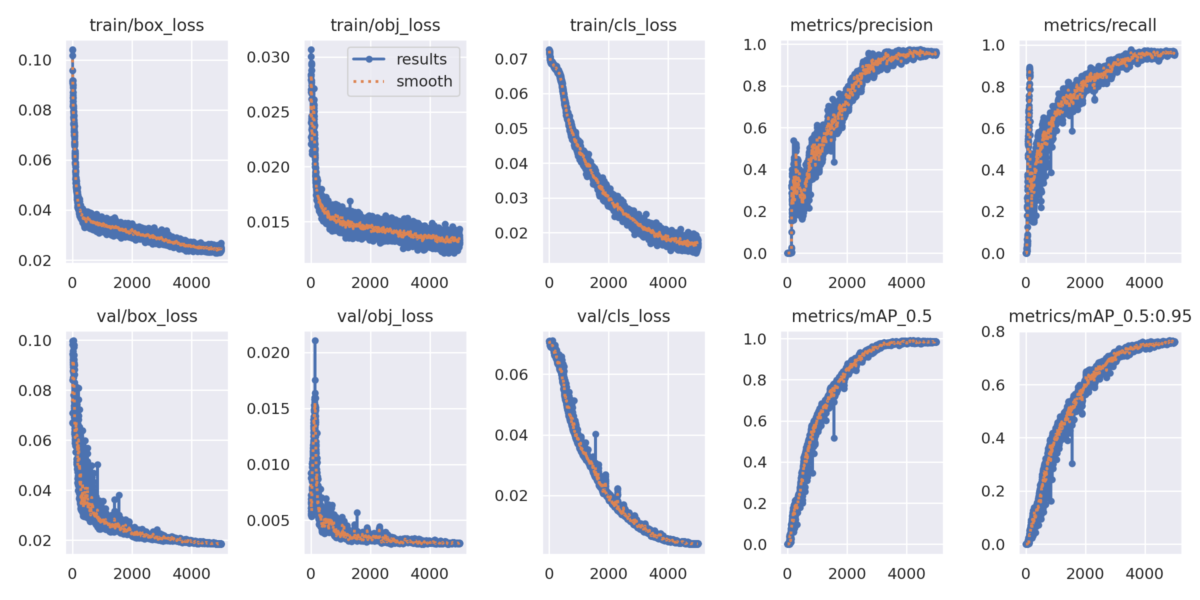
To verify the effectiveness of this convolution kernel in real-world scenarios, we conducted rigorous comparative experiments under controlled conditions.
Experimental Setup:
Dataset: Custom detection dataset (including highly similar categories such as batons, flashlights, and knives).
Training Strategy: SGD optimizer, Cosine LR scheduler, training for 5000 Epochs (to ensure full convergence).
Baseline: Only replace this module with a standard 3x3 DWConv, keeping the rest of the network architecture exactly the same.
4.1 Overall Performance Evaluation: Trade-off Analysis
COMMON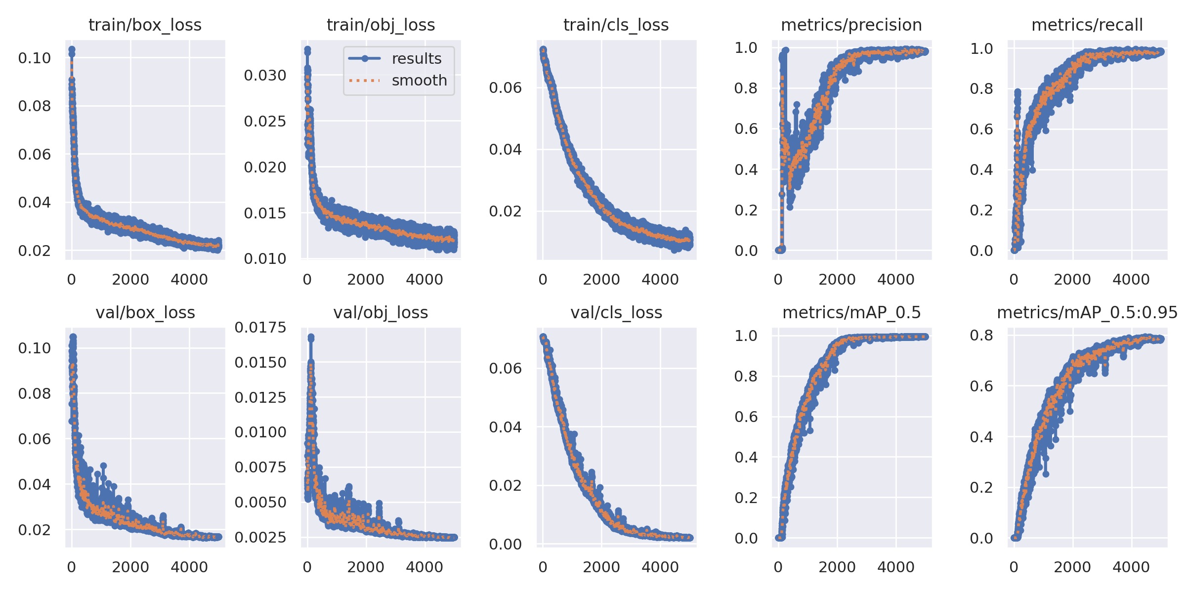
ENHANCE
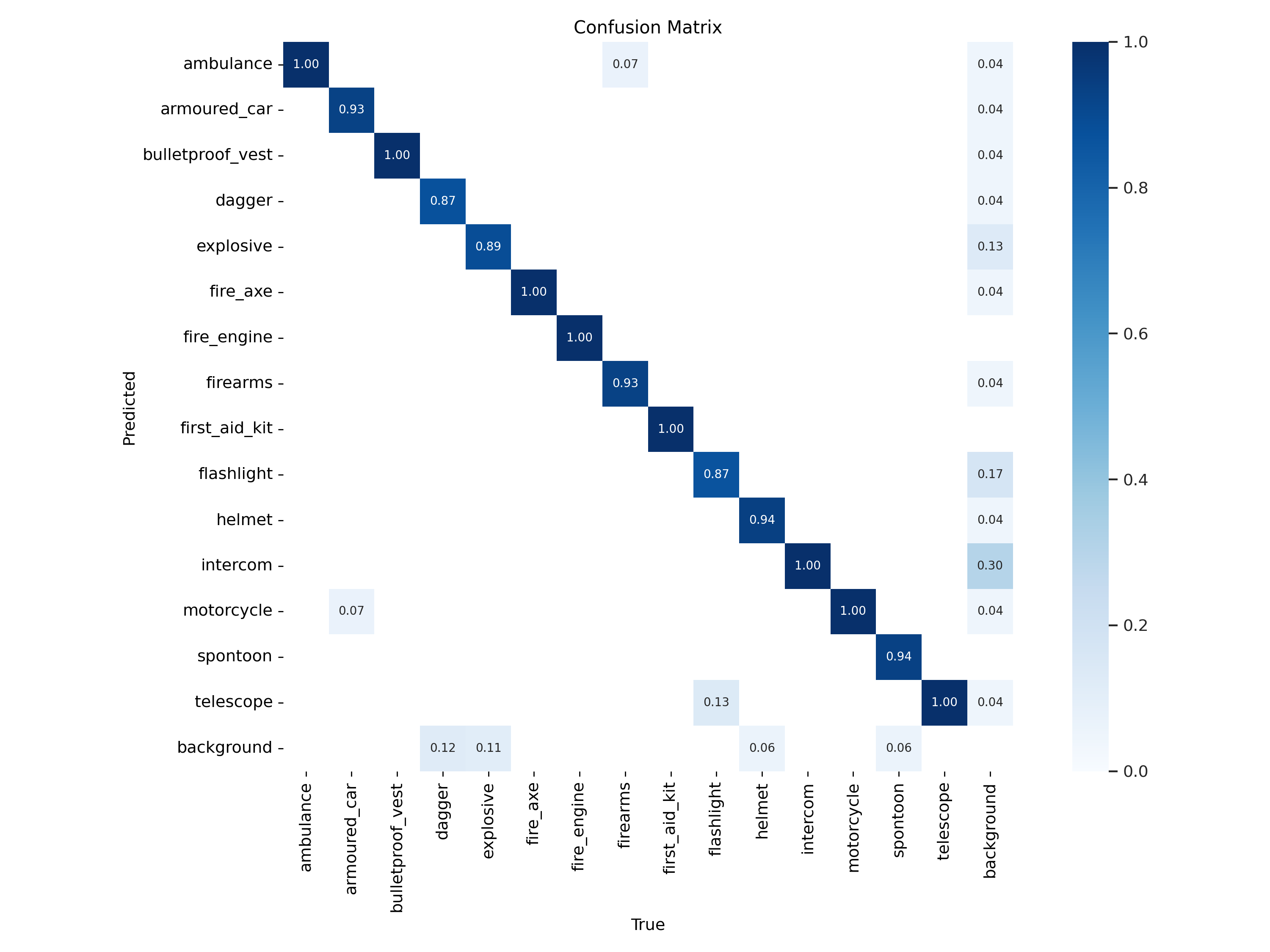
4.2 Hard Example Mining and Fine-Grained Classification
In testing, "inter-class similarity" is the biggest challenge.
For example, elongated "batons" and "flashlights" are extremely difficult to distinguish at low resolutions.
We extracted the model's Top-1 Accuracy on these specific categories for comparative analysis:
COMMON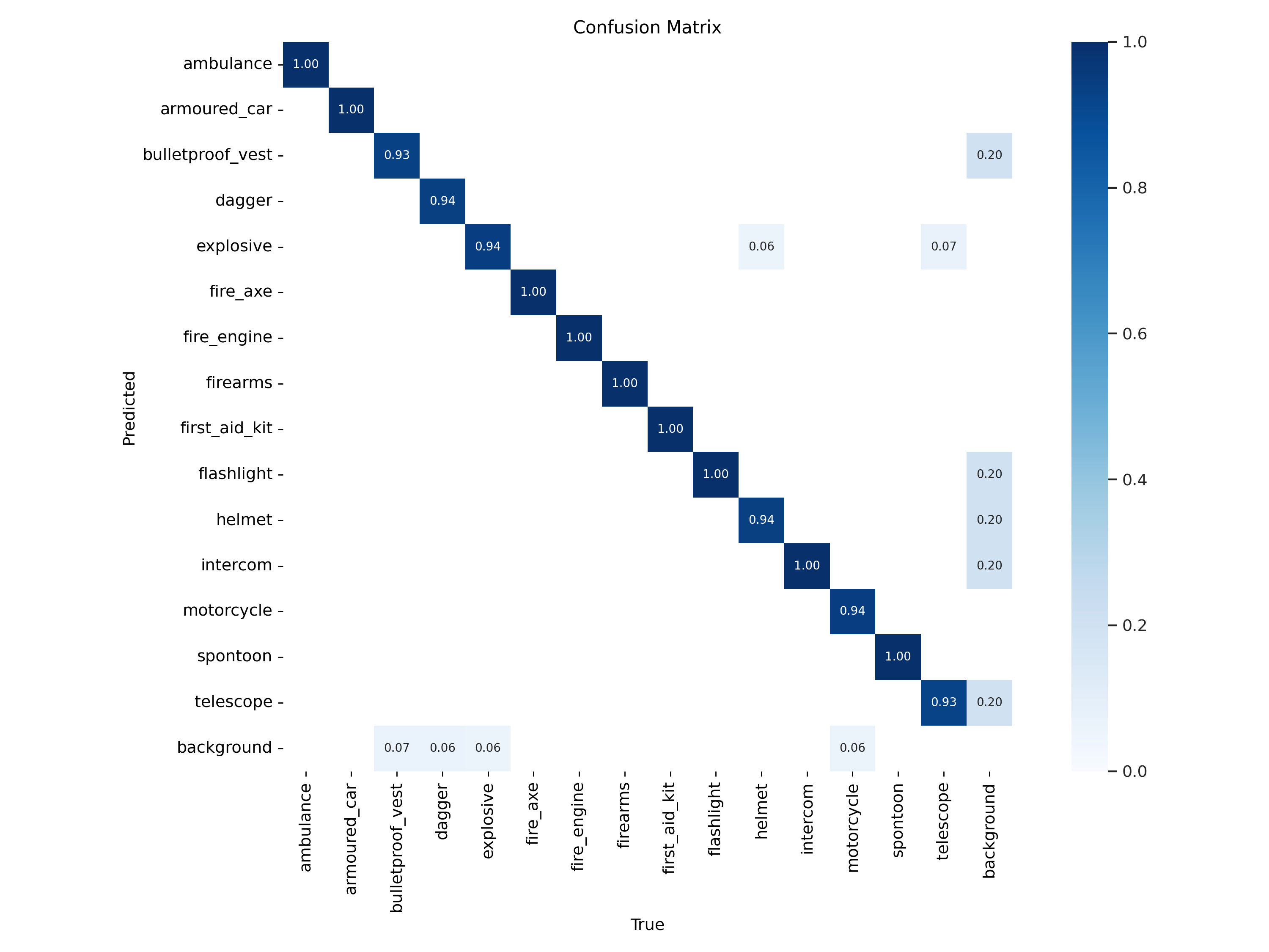
ENHANCE
5. Conclusion
This operator demonstrates a highly forward-looking approach to lightweight network design.
- It introduces stronger spatial inductive bias through convolutions.
- It solves the problem of standard CNNs lacking positional awareness through coordinate attention.
- It showcases excellent engineering implementation awareness through GroupNorm and Hardswish, making it highly practical for small-sample fine-tuning and edge inference scenarios.
This module is not just a plug-and-play component; it also provides a standard spatial-channel decoupling paradigm for future lightweight detection network design.